Quick Start • Single Cell Pathway Analysis (SCPA)

1. Broad overview of the workflow

pathways <- msigdbr("Homo sapiens", "H") %>%
  format_pathways()

# The populations here just need to be your normalized expression matrices

scpa_out <- compare_pathways(samples = list(population1, population2),
                             pathways = pathways)

# For faster analysis with parallel processing, use 'parallel = TRUE' and 'cores = x' arguments

In this output, the qval should be the primary metric that is used to interpret pathway differences i.e. a higher qval translates to larger pathway differences between conditions. If only two samples are provided, a fold change (FC) enrichment score will also be calculated. A large advantage in assessing the multivariate distribution of a pathway in SCPA is that there will be pathways that show large qvals, but relatively small fold changes. These pathways therefore show large differences that are independent of mean changes in gene expression. These are still highly relevant pathways, which we show in our paper, and is why we suggest solely using the qval for your statistical interpretation.

2. Full workflow on an example dataset

Here we’re just going to show some general principles of what you need to get started in a basic pathway analysis. It acts as a quick reference to all the main points of the workflow, but more detailed examples can be found in our other tutorials.

Basic information needed for pathway analysis

The two main bits of information we need are:

Expression matrix for each condition (this can be formatted as separate data frames/matrices, or stored within a typical Seurat/SingleCellExperiment object)
Gene sets

Loading in packages

For this simple example, we’re going to load in a few packages. msigdbr allows access to a large number of gene sets that are collated here

library(SCPA)
library(msigdbr)
library(Seurat)
library(dplyr)
library(ggplot2)

Loading in data

Here we’re going to use data taken from the Szabo, P… Sims, P paper. You can find this data in an R object here

t_cells <- readRDS("szabo_t_cell.rds")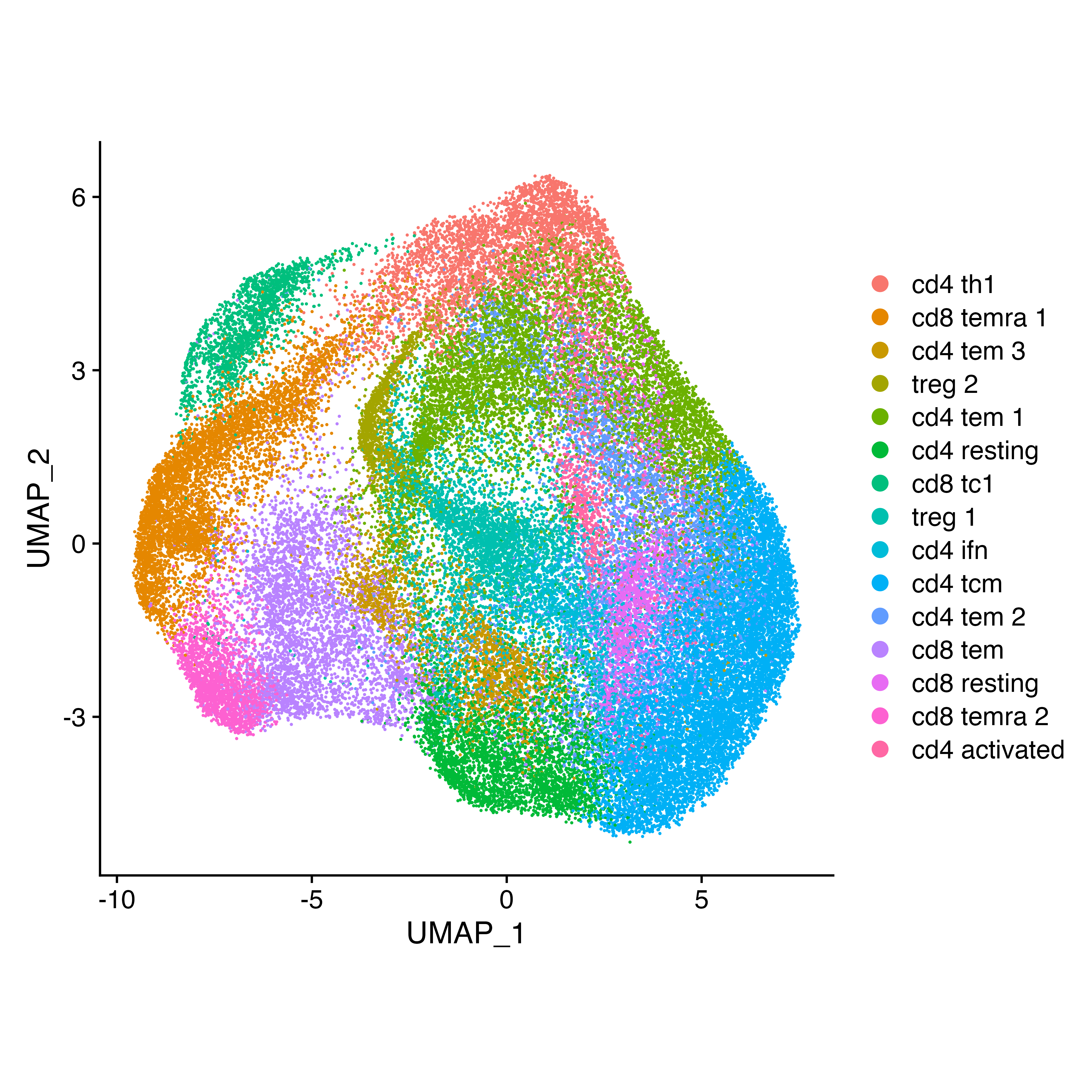

Quick Look at the data

DimPlot(t_cells) +
  theme(aspect.ratio = 1)

Generating samples from a Seurat object

For this basic comparison, we’re going to look at T helper 1 (Th1) and T central memory (Tcm) cells. To generate expression matrices that SCPA can use, we can run the seurat_extract function. This takes a Seurat object as an input, subsets data based on the Seurat column metadata, and returns an expression file for that given subset. If you have a SingleCellExperiment object, you can use the sce_extract function.

tcm <- seurat_extract(t_cells,
                      meta1 = "cell", value_meta1 = "cd4 tcm")
th1 <- seurat_extract(t_cells,
                      meta1 = "cell", value_meta1 = "cd4 th1")

Generate some gene sets using msigdbr

We then need to generate our gene sets. msigdbr is a handy package that allows you to get this information. Here we’re pulling all the Hallmark pathways, and using the format_pathways function within SPCA to get them properly formatted. A detailed explanation of generating gene sets for SCPA can be found here

pathways <- msigdbr("Homo sapiens", "H") %>%
  format_pathways()

Comparing samples

We’re all set. We now have everything that we need to compare the two populations. So just run compare_pathways and use the objects we created above.

scpa_out <- compare_pathways(samples = list(tcm, th1), 
                             pathways = pathways)

# For faster analysis with parallel processing, use 'parallel = TRUE' and 'cores = x' arguments

And in scpa_out, we have all our results.

head(scpa_out, 5)
#>                               Pathway          Pval      adjPval     qval
#> 32            HALLMARK_MYC_TARGETS_V1 5.788383e-101 2.894192e-99 9.926655
#> 2        HALLMARK_ALLOGRAFT_REJECTION  7.532277e-93 3.766139e-91 9.509159
#> 31          HALLMARK_MTORC1_SIGNALING  7.532277e-93 3.766139e-91 9.509159
#> 36 HALLMARK_OXIDATIVE_PHOSPHORYLATION  1.061001e-89 5.305003e-88 9.342126
#> 23       HALLMARK_IL2_STAT5_SIGNALING  1.315549e-86 6.577745e-85 9.175071
#>           FC
#> 32 -87.81108
#> 2  -21.07656
#> 31 -45.82991
#> 36 -47.98635
#> 23 -20.23701

Plotting some basic output

You can use SCPA to generate a pathway rank plot. For example, we can highlight one of the topmost pathways – MTORC1 – using the plot_rank function.

plot_rank(scpa_out = scpa_out, 
          pathway = "MTORC1", 
          base_point_size = 2, 
          highlight_point_size = 3)