Comparing two populations • Single Cell Pathway Analysis (SCPA)

Here we’re going to do a basic comparison of pathways between two populations using our naive CD4⁺ T cell dataset that you can find here.

Let’s load in a few packages we’ll need

library(SCPA)
library(Seurat)
library(tidyverse)

Loading in data and visualizing

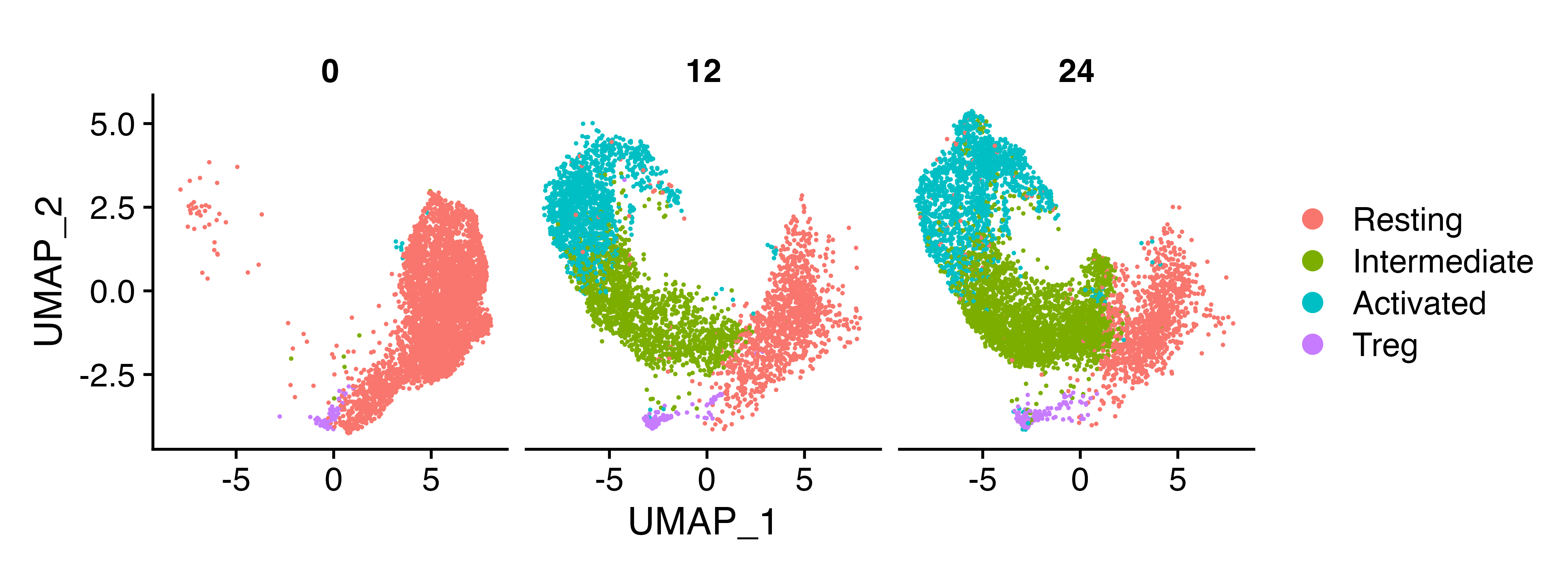
And let’s load in the data we’re going to use. In this dataset, CD4⁺ T cells were left unstimulated, or stimulated for 12 or 24 hours with anti-CD3 and anti-CD28

naive_cd4 <- readRDS("naive_cd4.rds")

In the naive_cd4 object, we have all our naive CD4⁺ T cells with metadata specifying the identified cell types and the hour specifying time point of cell harvesting.

DimPlot(naive_cd4, split.by = "Hour") +
  theme(aspect.ratio = 1)

Extracting the expression matrices

We then need the expression matrices for the populations we want to compare. For this, we can use the seurat_extract function from the SCPA package, which takes a Seurat object and subsets the data based on the metadata specified in the Seurat columns e.g. here we want to take ‘Resting’ cells at 0hr, and ‘Activated’ cells at 24hr. If you have a SingleCellExperiment object, you can use the sce_extract function.

resting <- seurat_extract(naive_cd4,
                          meta1 = "Cell_Type", value_meta1 = "Resting",
                          meta2 = "Hour", value_meta2 = 0)

activated <- seurat_extract(naive_cd4,
                            meta1 = "Cell_Type", value_meta1 = "Activated",
                            meta2 = "Hour", value_meta2 = 24)

Defining metabolic pathways

After we have our data, we can define the pathways to compare. We curated a list of metabolic pathways from a few different sources (Hallmark, KEGG, and Reactome), which can be found here. The file is in standard gmt file format with the pathway name in column 1 and genes of that pathway in subsequent columns. Here we just converted a gmt file to csv, and manually curated a single file with all metabolic gene sets. SCPA just needs the filepath to these gene sets, so we can add this as an object to simplify our final chunk of code

pathways <- "combined_metabolic_pathways.csv"

Running SCPA

So now we have our samples and metabolic gene sets. To compare these pathways, we can just run the compare_pathways function.

rest_act <- compare_pathways(samples = list(resting, activated), 
                             pathways = pathways)

# For faster analysis with parallel processing, use 'parallel = TRUE' and 'cores = x' arguments

Visualizing results

Now we have the results stored in the rest_act object, which we can then visualize.

rest_act <- rest_act %>%
  mutate(color = case_when(FC > 5 & adjPval < 0.01 ~ '#6dbf88',
                           FC < 5 & FC > -5 & adjPval < 0.01 ~ '#84b0f0',
                           FC < -5 & adjPval < 0.01 ~ 'mediumseagreen',
                           FC < 5 & FC > -5 & adjPval > 0.01 ~ 'black'))

aa_path <- rest_act %>% 
  filter(grepl(pattern = "reactome_arachi", ignore.case = T, x = Pathway))

ggplot(rest_act, aes(-FC, qval)) +
  geom_vline(xintercept = c(-5, 5), linetype = "dashed", col = 'black', lwd = 0.3) +
  geom_point(cex = 2.6, shape = 21, fill = rest_act$color, stroke = 0.3) +
  geom_point(data = aa_path, shape = 21, cex = 2.8, fill = "orangered2", color = "black", stroke = 0.3) +
  xlim(-20, 80) +
  ylim(0, 11) +
  xlab("Enrichment") +
  ylab("Qval") +
  theme(panel.background = element_blank(),
        panel.border = element_rect(fill = NA),
        aspect.ratio = 1)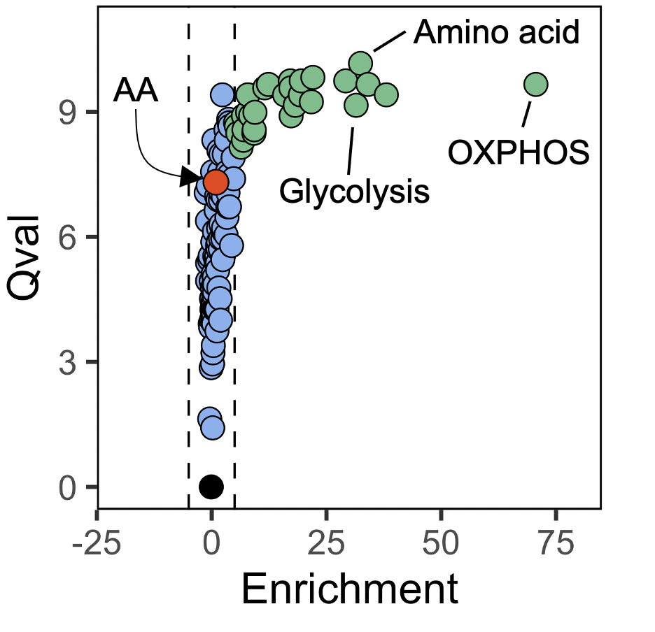

Some conclusions about SCPA

An important aspect of SCPA is highlighted here, in that pathways showing large changes in multivariate distribution (i.e. pathway ‘activity’) do not always show mean changes. So looking at the plot, we see a large number of pathways that have high qvals, but no enrichment in any given population. In the plot above we highlight arachidonic acid as one particular pathway that shows this pattern, and in our wet lab work, we have shown that these pathways are also very relevant when understanding pathway importance (see figure 4 in our paper here . So here we suggest that the qval should be used as the primary statistic when judging biological relevance, and the pathway fold change/enrichment should only be a secondary informative value. For more on interpreting the output of SCPA, see this tutorial